DCOP graph models
When solving a DCOP, The first step performed by pyDCOP is to build a graph of computations. This computation graph must not be confused with the constraints graph ; while they may sometime be similar. The constraints graph is strictly a graph representation of the Constraints Optimization Problem (COP) while the computation graph depends on the method (aka algorithm) used to solve this problem.
A computation graph is a graph where vertices represent computations and edges represent communication between these computations. Computation send and receive messages one with another, along the edges of the graph. Computations are defined as the basic unit of work needed when solving a DCOP, their exact definition depends on the algorithm used. Most algorithms define computations for the decision variables of the DCOP, but some algorithm can define computations for constraints as well, or even groups of variables.
Pydcop defines at the moment 3 kinds of computation graphs:
Constraints hyper-graph
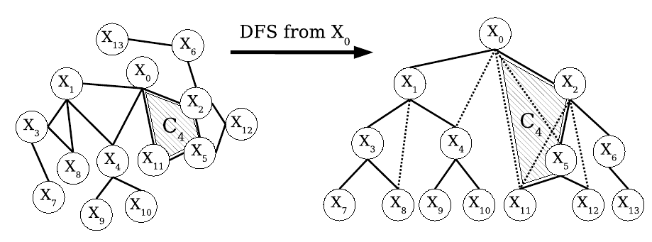
Pseudo-tree (aka DFS Tree)
Factor graph
When solving a DCOP, as each algorithm require a specific type of graph, pydcop can automatically infer the computation graph model from the algorithm you’re using.
Constraints hyper-graph
This is the most straightforward computation graph and is used with algorithms that define one computation for each variable. In a constraints graph vertices (i.e. computations) directly maps to the variables of the DCOP and edges maps to constraints. As a classical constraint graph can only represents binary constraints, pyDCOP uses an hyper-graph, where hyper-edges can represent n-ary constraints.
Factor graph
A factor graph is an undirected bipartite graph in which vertices represent variables and constraints (called factors), and an edge exists between a variable and a constraint if the variable is in the scope of the constraint.
Factors graph are used for algorithms that define computations for variables and for constraints. This is typically the caase of MaxSum and most GDL-based algorithms.

DFS tree
DFS trees are a subclass of pseudotrees, built a depth-first traversal of the constraint graph (where vertices represent variables and edges represent constraints). In addition to the parent/children edges of the tree, they contains pseudo-parent/ pseudo-children edges, which correspond to the edges (aka constraints) of the orginal graph that would othrwise not be represented in a simple tree.
The only algorithm currently implemented in pyDCOP that uses a DFS tree computation graph is DPOP
Implementing a new graph model
A module for a computation graph type typically contains
class(es) representing the nodes of the graph (i.e. the computation), extending ComputationNode
class representing the edges (extending Link)
a class representing the graph
a (mandatory) method to build a computation graph from a Dcop object :
def build_computation_graph(dcop: DCOP)-> ComputationPseudoTree: